Tag: science

Tensor Product Attention: Curiosities abound
A recent paper Tensor Product Attention Is All You Need¹ grabbed my attention. Over the last year, I have been exploring and investigating ways to reinterpret attention mechanism, mainly for my own edification. What correlations do a transformer really capture? And unsurprisingly, I have been looking at using intuition from the physics of correlated systems.

Firstly, attention mechanism is often written in a mathematically confusing and redundant way in the machine learning literature. The notation is often obfuscated by implementation quirks of matrix multiplications on GPUs. So let’s set up the notation, and simplify.

In the notes below, I will ignore position encoding. RoPE or learnable additive position encodings do not change the foundational mathematical intuitions I am trying to convey here — it is a distraction.

I use $\ell$ for layer index and $h$ for head index.

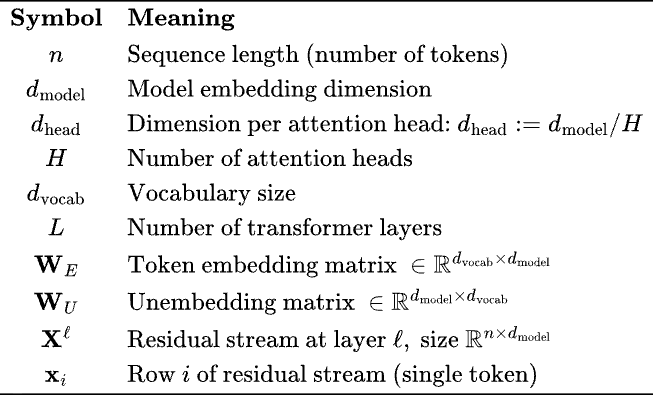
The key quantity is the residual stream, $X^\ell$ . This matrix is getting transformed by attention and MLP blocks. The embedding dimension $d_\textrm{model}$ is the size of the vector space in which tokens are being embedded.

We need a few other matrices to really explain what’s going on.

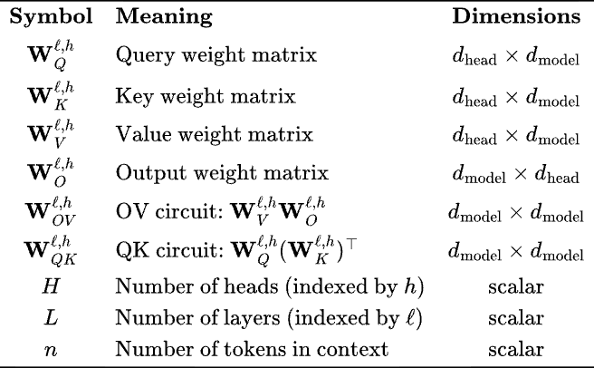
Note that in ML/ AI papers the Query, Value and Key matrices are always written separately, but in essence, we are low-rank decomposing (as product of rectangular matrices) two matrices, $\mathbf{W}_{QK}^{\ell,h} \, \, , \mathbf{W}_{OV}^{\ell,h}$ . This will be clear when we write attention is terms of these matrices —

$\begin{aligned} \text{Attn}^{\ell}(\mathbf{x}_i) = \sum_{h=1}^{H} \sum_{j=1}^{n} \left[ \text{softmax}_j \left( \frac{\mathbf{x}_i^\top \mathbf{W}_{\text{QK}}^{\ell,h} \mathbf{x}_{j}}{\sqrt{d_{\text{head}}}} \right) \right] \mathbf{W}_{\text{OV}}^{\ell,h} \mathbf{x}_j \end{aligned}$

The attention operator $\textrm{Attn}^\ell$ at layer $\ell$ is a sum over individual attention heads, $h$ , with $H$ total heads. Note, here I choose to call the operator the net function that returns a vector of same size as $\mathbf{x}_i$ — one can choose to add this back to the residual $X^\ell$ . Some architectures do so, others send it through the MLP operator. There are a lot of different transformer architectures out there in the various LLMs, and for the purpose of this discussion, it’s unimportant. Moreover, the papers have a bewildering range of definitions of what part of is called attention, which is why I bored you with setting up notation. You are welcome.

Note that the number of heads and head dimensions are chosen such that we always have $d_{\text{model}} \times d_{\text{model}}$ matrices in the above expression.

The only correlation between tokens explored in an transformer is pairwise. The MLP operator acts on the per-token embedding $\mathbf{x}_i$ and do not mix $\mathbf{x}_i$ and $\mathbf{x}_j$ . In the Attention operator $\textrm{softmax}_j$ term is a normalized weight — and every other token embedding $\mathbf{x}_j$ in the context window is getting summed over by this weight multiple by a linear transformation matrix. It is really quite simple.

Well, one may wonder — why only pairwise correlations? And, why only the above functional form for pairwise correlations?

A digression — for physicists like me, any time we see pairwise correlations, we think about Potts model, a generalization of the Ising Model which is perhaps better known. In the q-state Potts model the “spins” are unit vectors that point in q symmetric directions of a hypertetrahedron in q-1 dimensions, see here². In the classical Potts model these vectors interact only if their “spins” (state) are the same.

Can we draw an analogy with Potts Model? Yes, of course! Well, a paper³ already did a version of it—with a Potts Model where the interactions are not restricted to same “spins” but mix “spins”. It’s an enticing direction to study the dynamics of transformers using such mappings.

OK, end of digression.

The Memory Bottleneck in Modern Transformers

Large language models face a critical scalability challenge: the Key-Value (KV) cache. During autoregressive generation, standard Multi-Head Attention (MHA) stores keys and values for all previously generated tokens, consuming memory that grows linearly with sequence length:

$\text{Memory}_{\text{MHA}} \sim n \times H \times d_\text{head}$

See table to to recall notation. For a model with $H = 32$ and $d_\text{head} = 128$ processing a $n = 10^5$ token context, this amounts to over 800MB just for the KV cache of a single layer!

The fundamental question is whether we must store the full $H \times d_\text{head}$ representation for each token, or whether a more compact factorized representation can capture the essential structure with minimal information loss.

Tensor Decompositions: A Primer

Before diving into Tensor Product Attention (TPA), we need to understand the landscape of tensor decomposition methods. A tensor is simply a multi-dimensional array—scalars are 0-order tensors, vectors are 1st-order, matrices are 2nd-order, and so on.

CP Decomposition (CANDECOMP/PARAFAC)

The most common Tensor Decomposition is probably the CP decomposition.

Definition (CP Decomposition): A third-order tensor $\mathcal{X} \in \mathbb{R}^{I \times J \times K}$ has a rank- $R$ CP decomposition if it can be written as:

$\mathcal{X} = \sum_{r=1}^{R} \mathbf{a}_r \circ \mathbf{b}_r \circ \mathbf{c}_r$ where $\mathbf{a}_r \in \mathbb{R}^I$ , $\mathbf{b}_r \in \mathbb{R}^J$ , $\mathbf{c}_r \in \mathbb{R}^K$ and $\circ$ denotes the outer product.

Element wise, Equivalently, for indices $i,j,k$ :

$\mathcal{X}_{ijk} = \sum_{r=1}^{R} a_{ir} b_{jr} c_{kr}$

The CP decomposition represents a tensor as a sum of rank-1 tensors (outer products of vectors). This is the natural generalization of matrix SVD to higher orders, though unlike SVD, computing the optimal CP decomposition is NP-hard. Yeah, sucks, right?

Tucker Decomposition

Another popular tensor decomposition method is the Tucker Decomposition.

Definition (Tucker Decomposition): A Tucker decomposition factorizes a tensor into a core tensor $\mathcal{G} \in \mathbb{R}^{R_1 \times R_2 \times R_3}$ and factor matrices along each mode: $\mathcal{X} = \mathcal{G} \times_1 \mathbf{A} \times_2 \mathbf{B} \times_3 \mathbf{C}$ where $\mathbf{A} \in \mathbb{R}^{I \times R_1}$ , $\mathbf{B} \in \mathbb{R}^{J \times R_2}$ , $\mathbf{C} \in \mathbb{R}^{K \times R_3}$ and $\times_n$ denotes the mode- $n$ product.

More directly, the decomposition is —

$\mathcal{X}_{p q r} = \sum_{i}^{R_1} \sum_{j}^{R_2} \sum_{k}^{R_3}\mathcal{G}_{i j k}\, \mathbf{A}_{pi} \,\mathbf{B}_{qj} \mathbf{C}_{rk}$

The Tucker decomposition generalizes CP by allowing a dense core tensor. Note that the the sizes $R_1, R_2, R_3$ is obviously within the sizes $I, J, K$ of the tensor dimensions— a common choice is $R_1 = R_2 = R_3 = \text{min} ( I, J, K)$ . When tensor $\mathcal{G}$ is super-diagonal (non-zero only when all indices are equal), Tucker reduces to CP.

Tensor Train Decomposition

The tensor decomposition most familiar to physicists is probably the tensor train decomposition.

Definition (Tensor Train): A tensor train (TT) or Matrix Product State (MPS) represents a $d$ -dimensional tensor as a product of matrices —

$\mathcal{X}_{i_1, i_2, \ldots, i_d} = \mathbf{G}^{[1]}_{i_1} \mathbf{G}^{[2]}_{i_2} \cdots \mathbf{G}^{[d]}_{i_d}$

where $\mathbf{G}^{[k]}_{i_k} \in \mathbb{R}^{r_{k-1} \times r_k}$ with $r_0 = r_d = 1$ . The parameters $\{r_1, \ldots, r_k, \ldots, r_{d-1}\}$ are called bond dimensions or TT-ranks.

This is the same structure used to represent quantum many-body states in physics.

Tensor Product Attention: The Core Claim

Now we arrive at the key contribution of the TPA paper. Instead of storing full query, key, and value matrices, TPA represents them using contextual low-rank factorizations.

Standard Multi-head Attention

For token $i$ with embedding $\mathbf{x}_i$ , layer $\ell$ and head $h \in \{ 1, \dots, H \}$

$\begin{align} \mathbf{q}_i^{\ell,h} = \mathbf{W}_Q^{\ell,h} \mathbf{x}_i \in \mathbb{R}^{d_{\text{head}}} \\ \mathbf{k}_i^{\ell,h} = \mathbf{W}_K^{\ell,h} \mathbf{x}_i \in \mathbb{R}^{d_{\text{head}}} \\ \mathbf{v}_i^{\ell,h} = \mathbf{W}_V^{\ell,h} \mathbf{x}_t \in \mathbb{R}^{d_{\text{head}}} \end{align}$

We can stack all the heads into matrices, note that now the matrices are not just weights, but weights multiplied by embeddings—

$\begin{equation} \mathbf{Q}_i = \begin{bmatrix} \mathbf{q}_i^1 \\ \mathbf{q}_i^2 \\ \vdots \\ \mathbf{q}_i^H \end{bmatrix} \in \mathbb{R}^{H \times d_{\text{head}}} \end{equation}$

TPA

TPA factorizes the stacked query/key/value matrices as rank- $R$ sums of outer products.

$\begin{equation} \mathbf{Q}_i = \frac{1}{R_Q} \sum_{r=1}^{R_Q} \mathbf{a}^Q_r(\mathbf{x}_i) \otimes \mathbf{b}^Q_r(\mathbf{x}_i) \in \mathbb{R}^{H \times d_{\text{head}}} \end{equation}$

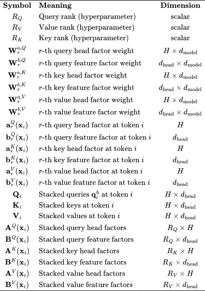
Note that the dimensions work out, for clarity —

$\begin{align} \mathbf{x}_i \in \mathbb{R}^{d_{\text{model}}} \quad \text{(input)} \\ \mathbf{W}^{a,Q}_r \mathbf{x}_i = \mathbf{a}^Q_r(\mathbf{x}_t) \in \mathbb{R}^{H} \quad \text{(head factor)} \\ \mathbf{W}^{b,Q}_r \mathbf{x}_i = \mathbf{b}^Q_r(\mathbf{x}_t) \in \mathbb{R}^{d_{\text{head}}} \quad \text{(feature factor)} \\ \mathbf{a}^Q_r \otimes \mathbf{b}^Q_r = \mathbb{R}^{H \times d_{\text{head}}} \quad \text{(outer product)} \\ \frac{1}{R_Q}\sum_{r=1}^{R_Q} \mathbf{a}^Q_r \otimes \mathbf{b}^Q_r \, = \mathbf{Q}_i \in \mathbb{R}^{H \times d_{\text{head}}} \quad \checkmark \end{align}$

So for standard MHA, each head independently projects the input—

$\begin{equation} \mathbf{q}_i^h = \mathbf{W}_Q^h \mathbf{x}_i \end{equation}$

whereas for TPA, all heads share $R_Q$ feature vectors, weighted differently per head,

$\begin{equation} \mathbf{q}_i^h = \frac{1}{R_Q} \sum_{r=1}^{R_Q} \underbrace{[\mathbf{a}^Q_r(\mathbf{x}_i)]_h}_{\text{head-specific weight}} \cdot \underbrace{\mathbf{b}^Q_r(\mathbf{x}_i)}_{\text{shared feature vector}} \end{equation}$

The Key Idea: Instead of H independent $d_\text{head}$ -dimensional vectors (one per head), TPA uses—
- $R_Q$ shared feature vectors $\mathbf{b}^Q_r \in \mathbb{R}^{d_{\text{head}}}$
- $R_Q$ weight vectors $\mathbf{a}^Q_r \in \mathbb{R}^H$ — one scalar per head, determining how much each head uses each feature
where $R_Q \ll H$ , therefore leading to parameter efficiency. Obviously, we have similar things going on for $\mathbf{K}_i$ and $\mathbf{V}_i$ .

Parameter counts

For MHA, we total number of parameters for queries only (similar for Keys and Values) are $H \times d_\text{head} \times d_\text{model} = d^2_\text{model}$

For TPA we have—
- Head factors: $R_Q$ matrices of size $H \times d_\text{model}$
- Feature factors: $R_Q$ matrices of size $d_\text{head} \times d_\text{model}$
- Total parameters— $R_Q (H + d_\text{head} ) d_\text{model}$
Example with typical paper values: $H=32$ , $d_{\text{head}}=128$ , $d_{\text{model}}=4096$ , $\boxed{R_Q=6}$ :
- MHA: $32 \times 128 \times 4096 = 16{,}777{,}216$ parameters
- TPA: $6 \times 4096 \times (32 + 128) = 3{,}932{,}160$ parameters
- TPA uses ~23% of MHA’s parameters
Note: Unlike LoRA which factorizes weights, TPA factorizes activations. This means the factorization is contextual—it depends on the input token $\mathbf{x}_i$ . It’s a very interesting idea in how to capture input-dependent structure while maintaining compression!

Memory Reduction

The major advantage claimed by the paper is the memory saving in KV cache. My interest in this paper is beyond this, to study other forms of attention, but it’s useful to note the memory arguments.

From standard MHA we have—
- Store $\mathbf{K}_i \in \mathbb{R}^{H \times d_{\text{head}}}$ and $\mathbf{V}_i \in \mathbb{R}^{H \times d_{\text{head}}}$
- Total: $2 \times H \times d_{\text{head}} = 2d_{\text{model}}$
TPA stores only the factors—
- Store $\{\mathbf{a}^K_r(\mathbf{x}_i)\}_{r=1}^{R_K}$ and $\{\mathbf{b}^K_r(\mathbf{x}_i)\}_{r=1}^{R_K}$ for keys
- Store $\{\mathbf{a}^V_r(\mathbf{x}_i)\}_{r=1}^{R_V}$ and $\{\mathbf{b}^V_r(\mathbf{x}_i)\}_{r=1}^{R_V}$ for values
- Total: $(R_K + R_V)(H + d_{\text{head}})$
The compression ratio is

$\rho = \frac{(R_K + R_V)(H + d_{\text{head}})}{2H \, d_{\text{head}}}$

Concrete example: $H = 32, d_{\text{head}} = 128, R_K = R_V = 1$ :
- TPA cache $= 2 \times (32 + 128) = 320$ values per token
- MHA cache $= 2 \times 32 \times 128 = 8192$ values per token
so TPA leads to $96 \%$ memory reduction! For context window of 100,000 tokens, MHA needs 1.6 GB of memory wheres TPA needs 64 MB of memory! (both per layer)

Connection to MPS

Another way to look at TPA is recasting it as a MPS. Per head, instead of the term $\mathbf{x}_{i}\mathbf{W}_{\text{QK}}^{\ell,h} \mathbf{x}_{j}$ in MHA, for TPA we have

$\begin{align} (\mathbf{q}_i^h)^\top \cdot \mathbf{k}_j^h = \left(\frac{1}{R_Q} \sum_{r=1}^{R_Q} [\mathbf{a}^Q_r]_h \cdot \mathbf{b}^Q_r\right)^\top \cdot \left(\frac{1}{R_K} \sum_{s=1}^{R_K} [\mathbf{a}^K_s]_h \cdot \mathbf{b}^K_s\right) \\ = \frac{1}{R_Q R_K} \sum_{r=1}^{R_Q} \sum_{s=1}^{R_K} ([\mathbf{a}^Q_r]_h \cdot \mathbf{b}^Q_r)^\top \cdot ([\mathbf{a}^K_s]_h \cdot \mathbf{b}^K_s) \\ =\sum_{r=1}^{R_Q} \sum_{s=1}^{R_K} \underbrace{[\mathbf{a}^Q_r(\mathbf{x}_i)]_h \cdot [\mathbf{a}^K_s(\mathbf{x}_j)]_h}_{\text{head-space mixing}} \cdot \underbrace{(\mathbf{b}^Q_r(\mathbf{x}_i))^\top \cdot \mathbf{b}^K_s(\mathbf{x}_j)}_{\text{feature-space contraction}} \end{align}$

We now we are getting somewhere, right? That’s a very different take on the attention matrix capturing token-token correlations!
- Rank indices $(r,s)$ play the role of bond indices in MPS
- $\sum_{r=1}^{R_Q} \sum_{s=1}^{R_K}$ is the bond cotraction
- Low ranks $R_Q, R_K$ is equivalent to low bond dimension and increased efficiency and high bond dimension leads to more expressiveness
Copy Tensor

We can look at the above expression in terms of copy tensors in Tensor Networks. A copy tensor⁴ allows for reusing information. For a vector $\mathbf{a} \in \mathbb{R}^d$ , the copy operation is represented by a diagonal tensor, $\mathcal{C}_{ij} = \delta_{ij}$ , the Kronecker delta. In other words, a copy tensor allows a single input to be reused in multiple tensor contractions.

Note what’s happening in TPA! The same input vector $\mathbf{x}_i$ is used $2 R_Q$ times for Query, and so on for Key and Value —

$\begin{align} \mathbf{x}_i \xrightarrow{\mathbf{W}^{a,Q}_1} \mathbf{a}^Q_1(\mathbf{x}_i) \in \mathbb{R}^H \\ \mathbf{x}_i \xrightarrow{\mathbf{W}^{b,Q}_1} \mathbf{b}^Q_1(\mathbf{x}_i) \in \mathbb{R}^{d_{\text{head}}} \\ \vdots \\ \mathbf{x}_i \xrightarrow{\mathbf{W}^{a,Q}_{R_Q}} \mathbf{a}^Q_{R_Q}(\mathbf{x}_i) \in \mathbb{R}^H \\ \mathbf{x}_i \xrightarrow{\mathbf{W}^{b,Q}_{R_Q}} \mathbf{b}^Q_{R_Q}(\mathbf{x}_i) \in \mathbb{R}^{d_{\text{head}}} \end{align}$

Instead of computing H independent projections (standard MHA), TPA computes $2 R_Q$ projections and cleverly recombines them. When $R_Q \ll H$ , this architecture is much more efficient while maintaining expressiveness of a Tensor Network (outer product).

Few other things…
- The paper shows that TPA is compatible with RoPE embedding. RoPE only acts on the $\mathbf{b}$ vectors. The keys are pre-rotated and stored, so no rotation is needed during decoding. Only the current query needs to be rotated. Neat!
- Remarkably, standard attention mechanisms are non-contextual variants of TPA! They show that both GQA (Grouped Query Attention) and MQA (Multi-Query Attention) are simply poor man’s version of TPA with $\mathbf{a}$ being independent of $\mathbf{x}_i$ !
I loved the paper. The key lessons:
1. Structure matters: Exploiting low-rank structure in attention patterns enables massive compression
2. Contextual factorization: Factorizing activations (not weights) is a very interesting concept
3. Model performance and memory needs: As with several other work recently, the belief that larger context window either means larger models, or we need to compromise on expressivity of the correlations captured in attention, may be incorrect
As we push toward longer contexts and larger models, principled compression techniques like TPA is a fruitful area of research. The tensor network perspective suggests we’ve only begun to explore the space of possible architectures!

References
1. Zhang, Yifan, et al. “Tensor product attention is all you need.” arXiv preprint arXiv:2501.06425 (2025). ↩︎
2. Wu, Fa-Yueh. “The Potts Model.” Reviews of modern physics 54.1 (1982): 235. ↩︎
3. Rende, Riccardo, et al. “Mapping of attention mechanisms to a generalized Potts Model.” Physical Review Research 6.2 (2024): 023057. ↩︎
4. Glasser, Ivan, Nicola Pancotti, and J. Ignacio Cirac. “From probabilistic graphical models to generalized tensor networks for supervised learning.” IEEE Access 8 (2020): 68169-68182. ↩︎
January 30, 2026
Carrier-free mRNA delivery with Aptamers: Nucleic acid is all you need
Folks who have been dreaming happily like I have over the past decade that nucleic acids are the right substrate for engineering medicines, well, here is one more evidence that we might just be right with our obsession with this marvelous polymer of life!

Here is how I evangelized my obsession amongst colleagues.

Silicon Valley is silicon valley and not germanium valley — germanium just wasn’t the right substrate though the first transistor was made of germanium after all, see here for the first paper and here for a lovely history of the transistor.

Aren’t you glad? — Germanium Valley just doesn’t quite have the right euphony, does it?

Nucleic acids are the right substrate for genetic and gene-centric medicines and I don’t think either small molecules or proteins are. Those are the germanium of genetic medicines — they may work but the sooner you use silicon the sooner we will solve all human diseases. Yeah, I am opinionated!

Circularized RNA + cell-type targeting aptamer

A fascinating paper quietly appeared on BioRxiv¹ about a month or so back. It’s a collaboration amongst multiple groups in China, with Weihong Tan as the PI.

They report first-in-human testing of very curious idea I had toyed with for a while now as a high-risk high-reward R&D project. They created aptamer-embedded circular RNAs (Apt-circRNAs). What’s wild is that they tested the concept in Phase 1 human trial right away from what would otherwise still be a marvelous proof-of-concept tested in ex vivo (blood) setting or in in vivo (humanized rodent) studies.

They got human clinical data. Wow!

The study combines two distinct and established ideas in nucleic acids—
- Circularizing of synthetic mRNA to enhance stability (the payload)
- Use of aptamers as a targeting molecule for cell-type specific delivery
This a totally crazy pace of testing out platform ideas. For those of you who do not work in the field — why is this significant?

Current mRNA vaccines like those for COVID-19 rely on LNPs for delivery, which can sometimes cause immunogenicity and predominantly accumulates in the liver. The Apt-circRNA platform is clever: the RNA molecule itself contains targeting information (receptor-targeting aptamers) to achieve cell-type-specific delivery, eliminating the need for synthetic carriers like LNPs to gift wrap the RNA.

The Three-Module Design

The Apt-circRNA platform elegantly integrates three functional modules into a single RNA molecule—

Targeting Module

The authors embedded dendritic cell (DC)-specific aptamers at precise locations within the circular RNA scaffold. They tested three targeting aptamers—nucleolin (nuc), transferrin receptor (waz), and DEC-205 (also called CD-205) (min2).
- Recall that DEC-205 (also called CD-205) is a cell surface-receptor (and endocytic receptor) highly expressed in immature Dendritic Cells (DCs).
- Transferrin receptor (TfR) is highly expressed in mature DCs and is crucial for iron uptake
- Nucleolin is also a cell surface receptor in endothelian cells and DCs. It can internalize from cell-surface to the nucleus
They used the Waz aptamer sequence for TfR—Waz was created by a Matt Levy whom I had hired at Creyon Bio, and who has lead the aptamer team and created a diversity of cell-type specific aptamers since. We know this aptamer well!²³⁴.

Waz aptamer sequence from Ref. 3

The Waz aptamer has chemical modifications as far as I remember—2’F modified C/Us and probably 2’OMe for some positions. The study uses native RNA—so there are no chemical modifications on the aptamer sequence. It’s an important distinction to keep in mind.

The DEC-205 aptamer min2 was also discovered my Matt’s group.⁵ The sequence from Fig.1 of Ref. 4 is —

Min2 aptamer Ref 4

The waz aptamer showed superior binding to both murine and human DCs. Through some optimization, the study determined that a bispecific combination of 5 waz and 4 min2 aptamers yielded optimal antigen presentation. Intersting! Thats a lot of aptamers decorating the RNA!

Stable expression framework

The circular RNA architecture provides inherent nuclease resistance by eliminating free 5’/3′ termini. The study demsntrates that the Apt-circRNA maintains structural integrity for over 24 hours and dramatically outperforming N1-methylpseudouridine-modified linear mRNA (m1Ψ-mRNA). This confirms older work that circularization of mRNA helps in extending half-life⁶⁷. The construct also remains stable across pH 4.0-8.0 which critical for endosomal trafficking.

Antigen-Encoding Region

An Internal Ribosome Entry Site (IRES) enables cap-independent translation, while codon-optimized sequences encode tumor-specific antigens. The modular design permits flexible incorporation of diverse antigens, demonstrated with ovalbumin peptides ranging from 8 to 386 amino acids.

The Clever Circularization Strategy

Here’s where the molecular engineering gets quite ingenious! The team adapted permuted intron-exon (PIE) ribozyme systems from two sources: Anabaena pre-tRNA and T4 bacteriophage td intron. The key innovation: they engineered the aptamer’s stem-loop structure to serve as the circularization site without mutating the aptamer sequence itself!

The process works by introducing a cleavage site within the aptamer’s loop region, then engineering the group I intron’s P1 and P10 guide sequences to complement sequences flanking the aptamer cleavage site. This enables precise, ribozyme-catalyzed splicing at the predefined loop site, generating Apt-circRNA products free of residual intron sequences.

Cute!

What’s the bio-distribution of Apt-circRNA?

PET Imaging reveals precise lymph node targeting!

They used radio-labeled Apt-circRNA and positron emission tomography (PET) to track spatial and temporal distribution.

PET imaging showed predominant renal accumulation with no notable off-target accumulation in liver, spleen, heart, or other major organs. This specificity is striking and addresses a major concern with LNP-based systems, which accumulate significantly in liver and spleen. The renal accumulation is perhaps owing to renal clearance of such a relatively smaller molecular weight payload?

They also ran Cy5-labelled study—6 hours post-injection revealed that cy5-labelled Apt-circRNA preferentially accumulated in dendritic cells compared to B cells and macrophages. Apt-circRNA was efficiently internalized by DCs at the injection site!

This contrasts sharply with LNP-circRNA, which primarily remained as intact nanoparticles near the injection site before uptake by both B cells and DCs within lymph nodes. This is consistent with the expectation that aptamer-mediated recognition enables direct DC internalization and lymph node trafficking.

The study also looked at immuno-stimulatory responses. Worth a read.

Surprisingly, Luminex assays revealed that Apt-circRNA elicited lower systemic levels of reactogenicity-associated chemokines and cytokines than LNP-circRNA except IL-12. Apt-circRNA also demonstrated reduced cytotoxicity in BMDCs (murine bone-marrow derived DCs) compared to LNP-circRNA. I would have expected the opposite—recall that native RNA could invoke innate response from pathways that sniff out cytosolic RNA.

First-in-Human Clinical Trial

The authors initiated a Phase I clinical trial at Zhejiang Xiaoshan Hospital with remarkable speed, testing Apt-circRNA-KR2 in healthy volunteers. Here KR2 refers to the RNA payload expressing the mutations (G12D and G12V) most common in KRAS gene. They want to elicit a T-cell response in KRAS-mutant cancer.

G12D and G12V are two of the most common single amino acid substitutions at codon 12 of the KRAS gene. The G12D indicates a substitution of the normal amino acid Glycine (G) with Aspartic acid (D) at position 12, while G12V indicates a substitution with Valine (V).

The trial enrolled 12 healthy volunteers total. Though a small cohort, it’s very encouraging!
- Single-dose escalation cohort: 9 volunteers received 50, 100, or 250 μg doses (n=3/group)
- Multi-dose cohort: 3 HLA-A*02:01 or HLA-A*11:01-positive volunteers received 250 μg on days 1, 7, and 13
- Only 1 of 12 participants experienced any adverse event—transient flu-like symptoms resolving within 12 hours
- Zero injection-site reactions (0/12)
- Zero grade ≥2 adverse events (0/12)
- All hematologic parameters, immune cell subsets, and cytokines remained within normal ranges through 180 days
The safety profile is quite surprising and compares very favorably to LNP-mRNA vaccines, which commonly cause injection-site reactions, fever and systemic symptoms.

High notes

Unlike previous ‘naked mRNA’ approaches that lack stability and targeting, it’s a clever idea to encode aptamer within the RNA sequence itself. However, I am not convinced this is necessary and it will prohibit chemical modifications that can stabilize the aptamer, increase affinity and half-life. One could conjugate the aptamer to the circular RNA and modularize the system further.

The dual aptamer strategy is definitely very interesting. The combination of waz (TfR-targeting) and min2 (DEC-205-targeting) creates a bispecific design that enhances both binding affinity and functional outcomes. Are these serving different purposes in directly the payload to endocytic compartments?

Manufacturing could be quite scalable, as is! The in vitro transcription and ribozyme-mediated circularization can be performed at scale without the complex formulation processes required for LNPs. The >80% circularization efficiency is commercially viable. Also, perhaps this advantage is a counter-point to the first point I made about chemically-modified aptamers, for which the aptamer would have to separately synthesized and somehow conjugated to the RNA at specific sites that does not disrupt expression. Moreover, with multiple aptamers to decorate the RNA, it’s messy. Efficiency and purity of product would be a challenge.

Cellular uptake was still a bit low, and I suspect this is because the aptamers were not really optimized. They took existing aptamer sequences and slapped it on. Flow cytometry data showed that even in draining lymph nodes only a fraction of DCs take up Apt-circRNA. This may necessitate higher doses or more frequent administration compared to LNP-formulated mRNA, partially offsetting the manufacturing advantages. But I strongly believe this is a solvable engineering problem.

Also, the naked RNA formulation and size leads to rapid renal clearance. One could incorporate sugar / lipid modifications to the construct but then the modules need to be separate—the circularized RNA and the aptamer (chemically modified and say, with added ligands like PEG attached, or albumin binding aptamers). Totally doable!

The bigger picture

For decades, the field has focused on engineering increasingly sophisticated nanocarriers—optimizing lipid chemistry, surface modifications etc. What is thought provoking here is, Why engineer a carrier when you can engineer the RNA itself?

It’s a tantalizing possibility—Nucleic acid is all you need.

References
September 17, 2025