
“The eye wink at the hand; yet let that be / Which the eye fears, when it is done, to see.” ~ Macbeth
Over the past year, I got really interested in a problem that I originally encountered in protein LLMs. Massive activation and outlier features: certain feature coordinates in transformers are outliers with massive values, irrespective of the token. In the original incarnation of the problem, these massive values let to rather ill-behaved latent space for protein design, where the putative latent space was created by some aggregation statistics over the layer-wise encodings of the protein.
But this problem exists in traditional LLM transformers too. My amazing collabroators Mausum, Vishal, Vraj and I have put out a recent preprint attacking this problem from a mechanistic stance.
The puzzle
A Transformer keeps a residual stream: one vector per token, of size 
In trained language models, a few coordinates of this vector take huge values. In the models we studied, the largest value is between hundreds to thousands of times the median coordinate size. Much more extreme values have been reported in the literature! These are called massive activations (MAs). They have practical costs. They make low-bit quantization hard. They shape how KV caches can be compressed.
The odd thing is how long they last. An MA usually appears in an early layer and stays massive until the end of the network. Every later attention head and FFN block could, in principle, learn a linear update that brings the value back to a normal range. None of them does. Why?
Earlier explanations focus on where MAs come from: attention sinks on the BOS token, low-cost storage on delimiter tokens, and FFN blocks that act as directional amplifiers (Sun et al., 2026). These explain how an MA is created. They do not explain why later layers do not correct them.
Reading and writing
Each block in a Pre-LN Transformer does two things with the residual stream. With 

Some weight matrices read from the residual stream:
- attention:
,
,
- FFN (SwiGLU):
,

Other matrices write back to it:
- attention:
- FFN:
For a linear map 
- Read-blindness. The coordinate lies in the right null space of
. Changing its value does not change the output. The block cannot see it.
- Write-blindness. The coordinate lies in the left null space of
To correct an MA, a block must be able to do both: see the value, and write an update that pushes against it. If either side is blocked, the correction cannot happen.
How we measure blindness
First we fix the set of massive coordinates. Let 


The results are robust to the choice of 
Next, for a read matrix 


![(0, 1]](https://s0.wp.com/latex.php?latex=%280%2C+1%5D&bg=ffffff&fg=000&s=0&c=20201002)

If every coordinate were treated the same, each score would be 


To compare MAs with the other coordinates, we use a one-sided Mann–Whitney test and report the rank-biserial effect ![r_b \in [-1, 1]](https://s0.wp.com/latex.php?latex=r_b+%5Cin+%5B-1%2C+1%5D&bg=ffffff&fg=000&s=0&c=20201002)

We look at each block in two ways:
- Weight view. Use the trained weights alone.
- Operator view. Use second moments of real inputs and real residual updates on held-out text. This shows what the blocks do in practice.
Result 1: The read side is blind, the write side is open
We tested four models: Llama at 135M, 1.28B, and 2.56B parameters, and Qwen3 1.7B.
On the read side, 


On the write side, 

The MAs are also present at the block inputs after normalization. So the blindness comes from the learned read projections. Normalization does not remove the signal.
We propose the following asymmetry: later blocks do not read the MA value, so they cannot condition a correction on it, however, they still write to the MA coordinates, so the value can keep amplifying!
We postulate that token-independent feature values may be necessary to model language, but thier amplification is a unfortunate side effect of how the FFN and Attention operator works.
Result 2: The model adjusts if you close read blindness of an operator
Is any single read matrix necessary? We trained three variants of the Llama 1.28B model with the same hyperparameters:
| variant | change | perplexity | # MA coords | max MA |
|---|---|---|---|---|
| baseline | none | 14.21 | 10 |  |
| Frozen | random orthogonal, fixed | 14.67 | 7 |  |
| Reparam | kept orthogonal (Cayley) but trained | 14.24 | 10 |  |
| FFN Frozen |  orthogonal, fixed orthogonal, fixed | 13.67 | 11 | 681 |
An orthogonal
Freezing the FFN read projections gives the same pattern in the other direction. The FFN scores return to 0.50. Attention stays blind (

In all three variants, the write side stays open.
So no single read matrix carries the asymmetry. When one is forced open, the others take over. This result surprised us!
Result 3: what the FFN amplifier adds
Sun et al. (2026) describe the FFN write to coordinate 
![\displaystyle y_k(\tilde h) \approx \tilde h^\top S_k \tilde h, \qquad S_k = \frac12 (U_k + U_k^\top), \qquad U_k = \sum_i W_{\mathrm{down}}[k,i]\; W_{\mathrm{gate}}[i,:]^\top\, W_{\mathrm{up}}[i,:].](https://s0.wp.com/latex.php?latex=%5Cdisplaystyle+y_k%28%5Ctilde+h%29+%5Capprox+%5Ctilde+h%5E%5Ctop+S_k+%5Ctilde+h%2C+%5Cqquad+S_k+%3D+%5Cfrac12+%28U_k+%2B+U_k%5E%5Ctop%29%2C+%5Cqquad+U_k+%3D+%5Csum_i+W_%7B%5Cmathrm%7Bdown%7D%7D%5Bk%2Ci%5D%5C%3B+W_%7B%5Cmathrm%7Bgate%7D%7D%5Bi%2C%3A%5D%5E%5Ctop%5C%2C+W_%7B%5Cmathrm%7Bup%7D%7D%5Bi%2C%3A%5D.&bg=ffffff&fg=000&s=0&c=20201002)
Under their approximation, 


We asked what sets massive coordinates apart in this picture (Llama 1.28B):
| diagnostic | median on  | |
|---|---|---|
 | 7.74 | +0.78 |
 | 2.19 | +0.98 |
 | 0.39 | +1.00 |
within-set  | 0.53 vs 0.46 | — |
The amplifier directions of different massive coordinates are only a little more aligned than those of other coordinates (0.53 versus 0.46). They do not share one direction. What sets them apart is gain, and above all how much of the quadratic form sits in its top direction. That last ratio separates the two groups completely in this sample.
Why does the gain concentrate? We measured how concentrated each write row ![W_{\mathrm{down}}[k,:]](https://s0.wp.com/latex.php?latex=W_%7B%5Cmathrm%7Bdown%7D%7D%5Bk%2C%3A%5D&bg=ffffff&fg=000&s=0&c=20201002)
![\displaystyle \mathrm{IPR}\big(W_{\mathrm{down}}[k,:]\big) = \frac{\sum_i W_{\mathrm{down}}[k,i]^4}{\big(\sum_i W_{\mathrm{down}}[k,i]^2\big)^2} \in \big[1/d_{\mathrm{ff}},\, 1\big].](https://s0.wp.com/latex.php?latex=%5Cdisplaystyle+%5Cmathrm%7BIPR%7D%5Cbig%28W_%7B%5Cmathrm%7Bdown%7D%7D%5Bk%2C%3A%5D%5Cbig%29+%3D+%5Cfrac%7B%5Csum_i+W_%7B%5Cmathrm%7Bdown%7D%7D%5Bk%2Ci%5D%5E4%7D%7B%5Cbig%28%5Csum_i+W_%7B%5Cmathrm%7Bdown%7D%7D%5Bk%2Ci%5D%5E2%5Cbig%29%5E2%7D+%5Cin+%5Cbig%5B1%2Fd_%7B%5Cmathrm%7Bff%7D%7D%2C%5C%2C+1%5Cbig%5D.&bg=ffffff&fg=000&s=0&c=20201002)
Among massive coordinates, rows with higher IPR have larger
As I mentioned before, unfortunate side-effect!
Result 4: blindness comes first
We tracked 21 training checkpoints, from step 0 to step 20k, for the 1.28B model. We fixed the massive and control coordinates at the final checkpoint and traced them backward. For each signal, we recorded the first checkpoint where the two groups separate with 
- FFN read-blindness separates at 2.3k steps.
- FFN amplifier gain separates at 4.5k steps.
Caveat: The time ordering does not prove that blindness causes the amplifier, but provides circumstantial evidence that one dominates the other. The two parts play different roles. The amplifier explains how some coordinates receive very large FFN writes. Read-blindness explains why later blocks do not correct the values already there.
Result 5: training keeps it this way
Is the asymmetry an accident, or does training hold it in place? We used two local measures at the trained 1.28B checkpoint.
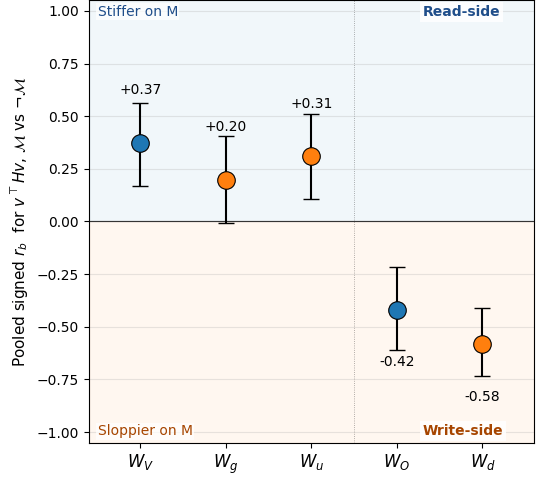
Curvature. For parameter slices tied to each residual coordinate, we sampled random unit directions 

We observe that read-side weights are stiffer on MAs. Write-side weights are sloppier. The loss holds the read-blindness in place more firmly than it holds the writes.
The next optimizer step. We applied one synthetic AdamW step at the trained checkpoint and computed its first-order effect on the size of each MA. The step increases MA size at every layer, with a larger effect in later layers. On matched non-massive coordinates the effect is near zero. Most of the increase comes from AdamW’s stored moment state. The new batch gradient has a much smaller effect. Weight decay pushes the other way, but the total effect is still an increase.
So at the end of training, the optimizer is still pushing massive activations to grow.
What this means
Massive activations persist because Transformers learn to ignore them when reading and keep adding to them when writing. This holds across scale (135M to 2.56B) and across two model families (Llama and Qwen3). The blindness is spread over several read matrices. Blocking it in one place moves it to another. The loss landscape and the optimizer state both support it.
Our guess about why: read-blindness is a cheap way for a model to keep token-independent features in the residual stream. Language modeling may need such features. The FFN quadratic amplifier and the lack of feedback control in write operations then push some of these features to massive values.
For anyone trying to remove MAs, for example to make quantization easier: changing one projection is not enough. Our interventions show the model routes around it.
More to come! Stay tuned! We are just getting warmed up!


Leave a Reply