We are called to be architects of the future, not its victims. The challenge is to make the world work for 100% of humanity in the shortest possible time, with spontaneous cooperation, and without ecological damage or disadvantage of anyone.
~ R. Buckminster Fuller
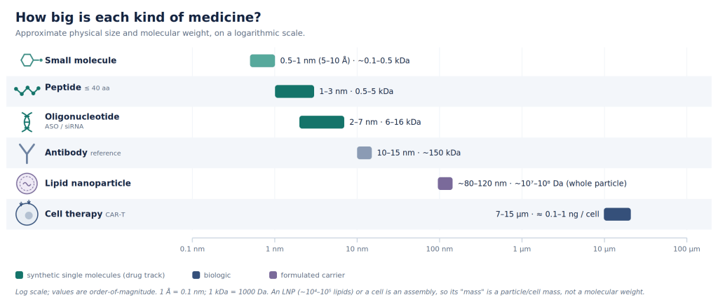
The human body is made from tens of trillions of cells drawn from roughly 400 distinct cell types. Most diseases manifest in only a small number of cells, and quite often in just a single tissue. However, the most common drug in our medicine cabinet are a class of molecules called small molecules. When swallowed or injected they reach almost everywhere and much of what we call a side effect of a drug is simply the result of its broad distribution to unintended cells and tissues.
A great deal of the art of medicine has always been a matter of bio-availability, for example, making sure the molecule crosses the gut and reaches the blood stream when taken orally.
The second most common drug modality after small-molecules is probably antibodies. They are rather large protein that was originally in the arsenal of our immune system, evolved to recognize a single protein among millions. Antibodies can be pointed at a target protein of our choosing, either to interfere with its function for therapeutic end, or as a targeting molecule that carries a payload for specific delivery. For example, fasten a toxin to antibody designed to target a receptor-protein and it finds the cancer cell, binds to the receptor-protein unique to that class of cells, delivers the poison to kill it, while leaving other cell types alone because they don’t express that specific receptor-protein. This is the antibody-drug conjugate (ADC), and over the past decade it has become one of the most successful ideas in cancer medicine.
At face value, the antibody is a superb targeting molecule. It binds its chosen target with great strength and precision, and we have learned, over forty years, how to create it. But it is also a large polymeric molecule made up of amino acid monomers and is quite hard to design. Over the last few years, AI tools for protein engineering (AlphaFold class of models) have revolutionized the field of de novo protein design. However, the design space is still enormous.
Let’s do the numbers. There are 20 natural amino acids. The naive space of design (all possible sequences) of length 100 is 20100 … or ~10130. As a reminder, there are 1080 atoms in the universe! Most antibodies are ~1000 amino acid long, though the variable region that is actually engineered is smaller. These variable domains (V) range in ~100 amino acids, Complementarity-Determining Regions (CDRs) is roughly 6-25 amino acids per loop, Single-Chain Variable Fragment (scFv) is ~240 to 260 amino acids, and Single-Domain Antibody (sdAb & nanobody) is ~110 to 130 amino acids. Still a very large design space!
Most importantly, antibodies are grown in cells, not synthesized: they are biologics. They are costly to produce: requiring expensive sterile bioreactors, nutrient-rich soup to feed engineered cells expressing them, and a lengthy purification and characterization process. Moreover, they are rather large molecules that may not reach certain biological compartments at all. (See Fig 1.)
The peptide and oligonucleotide polymer: so many control knobs!
Now imagine a short chain of amino acids (peptide), or a short strand of nucleic acids (oligonucleotide), synthesized one unit at a time in a machine. This is a synthetic, not a biologic. You choose every building block and you are not obliged to use natural amino acids/nucleic acids; you can use monomers nature never uses, alter the backbone, fold and clip the chain upon itself (called creatively, stapling and macro-cyclization), attach other chemical moieties. These functionalization strategies (chemical modifications to impart desired properties) are what makes it a fascinating engineering problem.
The number of molecules you can create this way is very large because your alphabet soup is much richer than the 20 canonical amino acids / 4 nucleobases. You have more control. The molecule is also shorter.
(For the astute reader: Nature does use a slightly larger class of building blocks than the 20/4. Cells orchestrate chemical modifications for both nucleic & amino acids, for example, methylation, glycosylation, phosphorylation etc.)
Proteins, however has a major advantage over peptides: availability of public data. The Protein Data Bank (PDB).
The PDB was built by publicly-funded science over several decades. The estimated cost to recreate it today is ~$20B! It has 3D structures of roughly 200K proteins, painstakingly characterized using NMR, cryo-EM or X-ray crystallography by hundreds of labs across the globe.
However, this amazing archive of structural biology is dominated by canonical amino acids. It does feature modified amino acids: ~1000 distinct ones. But these modifications appear in only 10% of the dataset, and mostly concentrated in just a handful of entries. The record barely touches the synthetic chemistries that peptide and oligonucleotide engineers actually use, for example, backbone surrogates, D-substitutions, and essentially the entire modified-oligonucleotide space.
So the hard part about peptides is not synthesis which has become rather routine and cheap. The hard part is knowing which ones have optimal pharmacological properties within an enormous and poorly charted space.
This problem of design and search is where computation is beginning to earn its keep.
But let’s dive a bit into the regulatory perspective first.
The dance of manufacturing and regulation
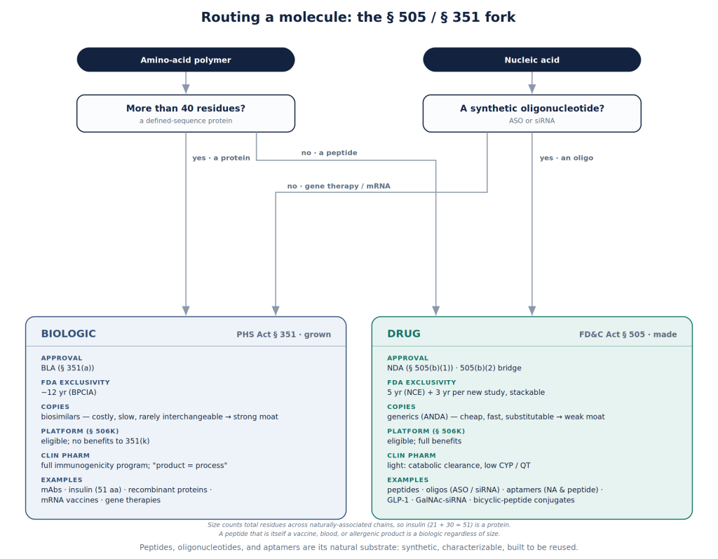
How a molecule is made turns out to matter far beyond the industrial process. A biologic is grown, and every batch carries the signature of the living system that produced it; unable to specify the product completely, the regulator treats the manufacturing process itself as part of the medicine. That is why a biologic has no true generic: a competitor cannot prove sameness, only similarity, and biosimilars may not be a real price competitor.
A synthetic peptide or oligonucleotide on the other hand is synthesized in defined chemical steps, and the same equipment, chemistry, and analytical methods serve the next molecule in the family. You change the sequence under the same process. The US Food and Drug Administration (FDA) has begun to call this a platform technology: a standardized way of making things that lets the knowledge begotten on one product — its manufacturing, its stability, its safety testing — carry over to the next. In recent guidance (the §506K designation program, and the 2026 roadmap urging sponsors to reuse prior knowledge to reach the clinic sooner) the agency provides some clarity on how it will recognize and reward platform efforts.
Synthetic peptides are short and fully specified. They sit on the drug side of the law (FD&C Act, §505 — NDA/ANDA) rather than the biologic side (PHS Act, §351 — BLA/bio-similar), and inherit the friendlier process: lighter clinical-pharmacology demands, a genuine generic pathway, and exclusivity a sponsor can stack across a program.
The flow chart below should help in understanding this.
Peptides and other polymers used as delivery molecules
It is tantalizing to imagine a world where a catalog of delivery molecules, tested clinically, can be used with any payload to deliver to any specific cells/ tissues. The payload could be an antibody, a small molecule or a nucleic acid. The payload could also be encapsulated in a Lipid Nanoparticle (LNP) which in turn is decorated by such a delivery agent.
Synthetics have the advantage here in that they could potentially achieve platform designation over a much larger diversity of molecules compared to biologics.
Biologics are not excluded from platform designation, however, what potentially gets such designation is narrow. The guidance’s monoclonal-antibody (mAb) example refers to the production line: the cell substrate, expression construct, and downstream purification shared by antibodies made the same way. The platform therefore spans a close family of similar molecules.
A synthetic delivery agent has huge advantages. Section 506K explicitly lists “molecular structure” and “delivery method” as technologies that can themselves be designated, and the guidance’s own example — a targeting moiety conjugated to a synthetic siRNA — notes that the moiety’s safety is unchanged across different payloads. Here the reusable element is the targeting molecule itself and the payload is potentially free to vary. The first type of platform would designate a way of making similar things while the second would define a way of aiming at many distinct cells and tissues.
There are several nuances here. The current regulatory landscape still treats the delivery molecule and its payload, joined together, as a new molecular entity (NME) that must be characterized across the standard preclinical and clinical measures of safety and efficacy, whether or not the payload had been approved on its own. This is because the conjugate may travel through the body differently, be cleared differently, or prove toxic in a way neither part was on its own. A platform does not remove that burden of proof, however, it reduces the need to re-establish the shared delivery agent each time it carries something new. The clinically-relevant R&D process is much cheaper and quicker.
Note: There is an upside in that burden-of-proof. A covalent conjugate is a genuinely new molecule. Therefore, it can qualify as a New Chemical Entity (NCE) and earn its own five years of exclusivity even when the payload alone was already approved. FDA grants this exclusivity only when the molecule’s active core is one it hasn’t approved before. Interestingly, even small covalent changes can create a distinct core. A delivery agent covalently joined to its cargo is almost certainly a NCE! (FDA however decides this case by case. It holds most clearly for covalent conjugates on the small-molecule drug track whereas biologics follow their own exclusivity rules.)
The current state of affairs in delivery molecules
Not surprisingly, today Antibody-Drug Conjugates (ADCs) dominate the field of targeted delivery. The space of synthetic polymers (peptides, oligonucleotides, sugars and lipids extensions) is evolving rapidly, and in my opinion holds the greatest promise in modularizing medicines and making them more precise.
Here are some existing examples:
| Molecule (company) | What the targeting solves | Status / 2024 sales |
|---|---|---|
| Pluvicto — ¹⁷⁷Lu-PSMA-617 (Novartis) | A PSMA-binding ligand delivers radiation only to tumor cells (a free radionuclide would be toxic for all cells) | Approved 2022; pre-chemo expansion Mar 2025; $1.4B, +42% |
| Lutathera — ¹⁷⁷Lu-DOTATATE (Novartis) | A somatostatin peptide carries radiation to neuroendocrine tumors | Approved 2018; ~$0.7B |
| GalNAc–siRNA — inclisiran (Novartis); givosiran, lumasiran, vutrisiran (Alnylam) | A small synthetic sugar routes siRNA into liver cells, turning otherwise-undeliverable siRNA viable (few-times-a-year subcutaneous dosing) | Approved 2019–22 |
| ADCs — Enhertu / T-DXd (AstraZeneca/Daiichi); Kadcyla / T-DM1 (Roche) | An antibody delivers a payload only to the tumor | Approved; Enhertu multi-$B, fast-growing |
| Trontinemab (Roche) | A transferrin-receptor brain shuttle carries an amyloid antibody across the blood–brain barrier — deep plaque clearance | Phase 3 (TRONTIER 1/2, from Sept 2025); rescued the failed gantenerumab binder |
The pattern is: a reusable delivery molecule (a sugar, a peptide, an antibody, a shuttle) plus a swappable payload. That is precisely the scaffold-plus-payload design FDA’s platform program was written to reward.
GalNAc is one of the most well-established examples. It is a small synthetic sugar that delivers genetic medicines to the liver (more precisely, ASGPR receptor). It is the existence proof that a synthetic delivery molecule can be equally good, if not better, when compared to antibodies. There are several other examples in the early clinical phases.
A synthetic delivery molecule would rescue or unlock a modality
Some medicines have sound biology and fail anyway because they cannot be delivered safely or at high enough concentration. A synthetic targeting molecule is often the missing piece.
| Modality | Delivery gap (with real stakes) | The targeting fix |
|---|---|---|
| Systemic AAV gene therapy (Zolgensma, Elevidys) | Dose-limiting, sometimes fatal liver toxicity (2025) | Muscle- and CNS-specific, liver-detargeted |
| Extrahepatic siRNA / ASO | Undeliverable outside the liver — no non-hepatic ligand at GalNAc’s efficiency | Muscle-, CNS-, and kidney-targeting peptide–oligo conjugates. |
| CAR-T / cell therapy | Ex vivo manufacturing cost. Cytokine-release and neurotoxicity | In vivo CAR generation with T-cell-targeted lipid nanoparticles |
| Radioligand therapy beyond PSMA/SSTR | Rate-limited by one high-affinity homing ligand per new antigen | New tumor-homing peptides |
| Cytokine therapy (IL-2, IL-12) | Severe systemic toxicity | Tumor-targeted or masked cytokines |
The cleanest example is in one company’s portfolio. Alnylam silences the same gene — transthyretin — in two approved drugs for the same disease. The first, patisiran, wraps the siRNA in a lipid nanoparticle given by IV infusion. The second, vutrisiran, carries an almost identical siRNA on a GalNAc conjugate injected under the skin once a quarter. The delivery molecule alone made the second drug simpler to dose and much longer-lasting.
The commercial prize
Many blockbusters have toxic side effects precisely because they reach everywhere in the body. Re-delivering the same molecule to its target tissue could widen the therapeutic window and, as the original drug lose intellectual property (IP) protection, create a new one.
Here is a summary of the comparisons I want to surface.
| Aspect | ADC (biologic) | Synthetic peptides & polymers |
|---|---|---|
| Targeting | Exquisite affinity and specificity, decades of validation | Emerging. Can be designed against many targets, very high affinities |
| Engineerability | Grown and selected. Design space is the complexity of proteins | Every unit specifiable, unnatural chemistry allowed, design space is compositional |
| Payload | Payload conjugation proven (the ADC for small molecules and siRNAs) | Any cargo (oligo, small molecule, radionuclide, antibody, mRNA) |
| Delivery architecture | Typically monovalent, few payloads | Direct conjugate, can be multivalent, or decorating a LNP/encapsulated carrier |
| Routes | Injection | More routes plausible, including oral |
| Manufacturing | Grown in living cells, lot-to-lot variability, CMC is very expensive | Machine-assembled, sequence-agnostic platform process, fully characterizable, CMC is much cheaper |
| Immunogenicity | Substatial and inherent | Lower for small molecules, chem. mods. can make immune-safe |
| Regulatory class | Biologic (§351): BLA; only biosimilar follow-ons | Drug (§505): NDA; true generics; 505(b)(2) bridges |
| Exclusivity / moat | ~12 yr, biosimilars barely erode price → strong moat | ~5 yr + stackable 3-yr, generics erode strongly → weaker moat |
| Platform-designation fit | Eligible, but benefits withheld from biosimilars | Strong; §506K’s own examples are a targeting moiety plus a swappable payload |
| Maturity | Mature, blockbuster | New frontier |
Summary
The antibody as of now has the better commercial shelter. However, the synthetic polymers are cheaper to make, far easier to engineer, somewhat indifferent to the cargo they bear, and favored in the modern manufacturing process and platform guidelines FDA has been whittling over the last few years.
But this is not a regulatory question alone, but a societal question. Do we want to make medicines precise?
The question that will decide how precise is our generation of precision medicine: which of the countless molecules we can design are the ones worth pursuing? How do we create the right catalogue of cell and tissue targeting agents in a reasonable time and cost?
Do we have courage to modularize medicine? Can we ever stop discovering them and graduate to engineering them? Can US biotech lead in this?
No other product in our lives, except for drugs, are still discovered. I am hopeful that we are the last generation when that is the case.
References
Primary regulatory sources (FDA / HHS). The regulatory argument in this essay rests on these documents:
- FDA, Platform Technology Designation Program for Drug Development — Draft Guidance for Industry, CDER/CBER, May 2024 (FD&C Act §506K). The platform-technology recognition and data-reuse argument.
- FDA, ANDAs for Certain Highly Purified Synthetic Peptide Drug Products That Refer to Listed Drugs of rDNA Origin — Guidance for Industry, CDER/OGD, May 2021. Synthetic peptides as drugs, and a genuine generic pathway.
- FDA, Clinical Pharmacology Considerations for Peptide Drug Products — Draft Guidance for Industry, CDER, December 2023. The lighter clinical-pharmacology burden.
- FDA, New Clinical Investigation Exclusivity (3-Year Exclusivity) for Drug Products: Questions and Answers — Draft Guidance for Industry, CDER, March 2026. Exclusivity a sponsor can stack across cohorts of a program.
- HHS, Operation TrialBlazer: HHS Roadmap to Maintaining U.S. Leadership in Early Clinical Research and Development, 2026. Reuse of prior and platform knowledge to speed early development.
- FDA Final Rule, Definition of the Term “Biological Product” — 85 FR 10057 (2020). The statutory drug-versus-biologic line drawn in Figure 1.